MonthJanuary 2016

2015 Winter Cryptography Project – P / NP, The Clique Problem

I recently read a book titled The Golden Ticket by Lance Fortnow in which the P / NP Problem and its importance to the theory of Computer Science are heavily discussed. Explained briefly, the P / NP Problem asks if every single problem can be solved quickly and efficiently. In relations to cryptography, P / NP is crucial because it allows for the creation of hard math problems to, for example, be able to hide private information on a public network. One of the most famous P / NP Problems, the Clique problem, was discussed and is, in my opinion, one of the more intriguing problems in the book.

Take, for example, a society called Frenemy, in which every citizen either has a 50% chance to be friends or a a 50% chance to be an enemy with a person they just met. In Fortnow’s book, he details how it would be virtually impossible to find all cliques of varying sizes (difficulty/time to find all cliques increases as size of desired clique increase) inside of this society (A clique is a group of people in which everyone is friends with all other members). At first, I didn’t think it would be that difficult to find the largest clique, but after making a simulation for myself, I was proven otherwise.

I stayed true to the Frenemy rules in my simulation – every time someone meets someone else, they have a 50% chance to either be their friend or their enemy. I experimented with varying population sizes as well as varying amounts of citizens in which each person can meet. I made two methods in order to experiment, one in which everyone meets everyone else in the society, and one in which everyone meets everyone on their own street (9 total streets in which 1/9 of the total population lives on each given street). To make the data easier to set up and understand, each citizen is given an identification number as well as an ‘address’, the number of street they live on. I aimed to find every single clique of size 3 in the society, and to see for myself how difficult it became to find them as population size increased.

Screen Shot 2016-01-13 at 1.49.10 PM

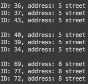
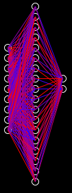
A couple of cliques present in a population size of 100 in which citizens met everyone on their own street.

I found that the total time to generate the population and find cliques of size 3 took much much longer the higher the population size was, which makes sense in hindsight. Adding a single citizen to a population size of 20 where everyone meets everybody doesn’t have nearly the impact as adding a citizen to a population size of 10,000,  as the number of updates a computer has to make to each citizen’s list of friends and enemies for a population of 10,000 is much larger. When I was reading Fortnow’s book, I didn’t put much thought into the rate at which the updates change as population size grows. I naively thought growth was generally linear, allowing total computations to find all cliques of size 3 to be relatively small compared to the actual value. Only after I made my own simulation did I truly understand the difficulty surrounding finding a solution to the Clique problem. If you find find yourself with some free time, I would recommend making a simple simulation like this for yourself so you can see the results firsthand.

I’d like to thank Lance Fortnow for pushing me to explore this problem through his book, as all P / NP problems (not just the Clique problem) are profoundly interesting in their own rights. And, if you’re planning to look more into the P / NP problem, Lance Fortnow’s The Golden Ticket is a must read. The discussion as well as the existence of the P / NP Problem has really expanded my understanding of Computer Science and the importance of not only the physical act of coding, but the theory behind CS as well.

2015 Winter AI/Arduino Project – Brainy Crawler

Having taken a general engineering course my senior year of High school at the same time I was researching Neural Networks (read more about Neural Networks here), I decided it was time to make a physical agent – a tangible robot controlled by a Neural Network. My background in robotics helped in this venture as well, as I knew before hand how servos and ultrasonic sensors worked.

Before getting to the hard part of writing the code to control the robot, I had to make the agent itself first. I knew I wanted to make a robot that learned how to move, but I didn’t have 2 motors. Instead, I decided to use servos, as it not only allows movement, but the motion itself is complex and warrants a fair amount of learning in order to master it. For parts, I used an Arduino Uno with 2 Parallax standard servos and 1 HC-SR04 Ultrasonic sensor. A friend of mine, Clay Busbey, helped out by 3D printing parts for me. I had 3 parts printed, the main chassis and 2 essentially straight bars used as 1 arm with a joint. I put the Arduino Uno and a half+ breadboard onto the chassis and hooked everything up from there.

crawler_png

Fritzing diagram of how I hooked up all of the components. It doesn’t show the bars used for arms, but you’ll see how that works in the next gif. The red and green LEDs indicate whether the Arduino is switching between Networks, red meaning it’s switching, and green meaning movements are controlled by a Neural Network.

In terms of the Neural Network, I used 3 input nodes, 1 hidden layer of 10 nodes, and 2 output nodes. The input values are the current position of each servo, along with the current distance away from the object detected in the ultrasonic sensor. The output values decide whether the servo should increase or decrease its current angle (> or < 0.5). I used a sigmoid function (1 / (1 + e^(-x))) as my activation function. Each Neural Network controls one motion, with a genetic algorithm that replaces the least successful Network (2 best networks make a crossover/mutation child that replaces worst network). Fitness is distributed based on how far the robot moved while under control of each Neural Network.

brainy crawler

Timelapse of the agent moving across the floor (sped up 3x). You can see that although it has a good start, it hiccups due to either a bad breed or mutation.

I enjoyed working on this project. It’s really one thing to watch a program learn in the real world as opposed to in the virtual world.

If you want to get the Arduino script and/or the .stl files for 3D printing the parts, you can get them here (.zip, 15 kb): https://drive.google.com/file/d/0Bz_0wgRmDpKqdGdGUS1YMk9oN1E/view?usp=sharing

2015 Winter AI Project – Evolution Simulator

The 2015 school year was when I began dabbling around AI. The idea always amazed me. Everything from movie depictions of them to the real practical uses they have in modern day life was interesting, and I wanted to know more about it.

Wanting to explore Neural Networks deeper (read more about Neural Networks here), I decided to make an evolution simulator. The aim of the project was to create a population of creatures that, starting with knowing nothing about their environment, evolved to chase after food and run away from predators. The creatures can also evolve different values of attack and defense, of which determines if that creature can eat other creatures. A set of 12 creatures is allowed to survive for as long as it can (must eat food to replenish a diminishing energy value, if it gets to 0 the creature dies), and at the end of the generation, the bottom half is eliminated, the top half reproduces sexually once (2 children) with each other (first mates with second, third mates with fourth, and so on), and asexually once as well. Reproduction is accomplished with crossover/mutation, that takes into account the weights for each creatures Neural Network and the attack value for each creature. Fitness is distributed based on how many times the creature eats.

The Neural Network itself was fun to make. I decided I wanted to make an adaptable system, that is, one in which I can change whenever I want it to. This includes the size of each individual layer and the total amount of hidden layers. For this project, I got the most success using one and two hidden layers with different amount of nodes for each (18 nodes for 1 layer, 5 nodes for 2 layers).

The input for each creature is as follows: 2 ‘eyes’ that take up 4 input nodes, as well as one node expressing the current angle the creature is facing. Each eye detects the angle from the creature to the closest entity (or second closest, for the second eye) and the r, g, and b values of that entity, expressed as a fraction over 255 (the range a color value can have is [0, 255]), allowing the creature to evolve decision making based on whether the entity it sees is edible or not. The output nodes control whether it turns left or right, and its velocity forwards or backwards (move more slowly while going backwards). I used a sigmoid function (1 / (1 + e^(-x))) as my activation function.

Screen Shot 2016-01-05 at 10.12.19 AM

Neural Network that has 9 input nodes, 1 hidden layer with 18 nodes, and 2 output nodes. The color for each weight is explained below.

Before I go over examples of the simulation, I’ll explain what each of the graphics in the frame represent. The creatures are represented by shades of purple (creatures that have a high defense are more blue while creatures that have a high attack are more red), with the current best creature (highest fitness) is outlined in yellow. The line extending from the center from each creature to its outline is the direction in which the creature is currently facing. Food is represented by the green squares. Moving onto the panels outside the main frame, the one in the top right shows the current generation, the amount of creatures alive (from a set max population size of 12), the best fitness value from the overall simulation, the best fitness value from the previous generation, and the best fitness for the current generation (represented with O, LR, and C respectively). The graphic below that panel displays the Neural Network of the creature that garnered the best fitness, where connections that are mostly red are between (0, 1), and connections that are mostly blue are between (-1, 0). Finally, the graph displayed on the bottom of the frame illustrates the best fitness for each round and shows overall growth of the population.

beginning

At the beginning, you can observe how most creatures are spinning out of control and lack in objective.

structured

After some time, you can see that although the creatures have not evolved the ability to go directly towards food, they have formed some structure in the way they collect it. You can also see that this population has evolved to contain creatures that have a high defense, as creatures that had a high attack in previous generations did not perform as well.

end usual

The usual ending. Creatures have evolved to not only go towards food, but to distinguish food from other creatures. That means that although an entity might be closer and thus more efficient to go towards, the creatures recognizes that entity as another creature and decides to go towards an entity that is further away because it recognizes that as food.

ending weird

Although creatures tend to evolve the ability to go straight for food, there are other strategies that have the possibility to emerge. For instance, in the simulation above, the creatures have come up with the strategy to propel themselves vertically, turn horizontally, and propel themselves the left or right whenever they detect food.

This project was incredibly fun to make. Although I had some frustration at the start while learning how to make Neural Networks of varying size, it  was fun finding solutions to my problems. I will probably keep working on this project for weeks or months to come, and I will definitely be utilizing my adaptive Neural Network on future projects.

If you want the source code, you can get it here (Java, 35 kb): https://drive.google.com/file/d/0Bz_0wgRmDpKqaXV0TVp0aXhIcTA/view?usp=sharing

© 2024 Brendan McCloskey

Theme by Anders NorénUp ↑