winter – Brendan McCloskey

Tagwinter

2018 Winter Data Analytics Competition – MCM

I took a brief break from working on side projects to participate in the MCM (Mathematical Contest in Modeling) competition. I decided to compete in this competition mainly after enjoying and seeing success in the previous semester’s GDMS data analytics competition (post linked here) in which my team received an honorable mention in the beginner’s division. Again, my team consisted of friends Kali Liang (CMDA major) and Eric Fu (BIT major). Looking back on both of these competitions, I would definitely say the diversity in majors really helped in our ability to come together and perform, mainly due to our differences in perspective when it came to looking at the problem as a whole. Similar to the previous competition, we were given a .csv file with about 600 categories involving energy consumption and production rates per year in Arizona, California, New Mexico, and Texas, and were asked to come up with energy profiles for each state and to predict energy consumption and production in 2025 and 2050, all in the context of using cleaner energy sources. For reference, we tackled problem C (all problems linked here).

We used a mixture of VBA (Excel), Python, and R to analyze the given data. My main job was to determine which subsets of data were interesting and useful and to plot them using Python/matplotlib.

Moving on to the actual data analysis, we started by creating energy profiles for each of the four given states. We split our profiles into 3 graphs we deemed relevant, including overall energy consumption, overall energy production, and energy usage by sector in each state. The main hurdle for this section was deciding how to cut down the data to where each graph wouldn’t be too cluttered but the data would still be accurate enough to use. For instance, for energy consumption alone, each state’s initial graph had over 20 sub-plots, making the graph hard to read at first glance. This was due to the inclusion of ultimately insignificant values (for instance wood and waste energy consumption). As a result, we cut these insignificant sub-sets, facilitating visual analysis on each graph. The downside to this was not having a fully accurate representation of total consumption and production in each state, but we decided the sacrifice was worth it for the visual clarity provided.
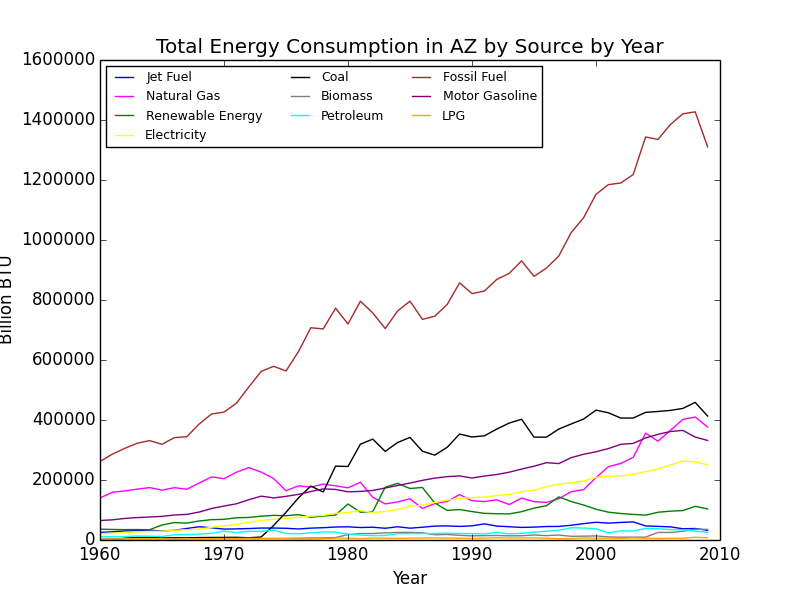
Energy consumption graph for Arizona. You can see that as the Y values approach 0, the higher the concentration of plot points (and this is after cutting more than 10 sub-sets).

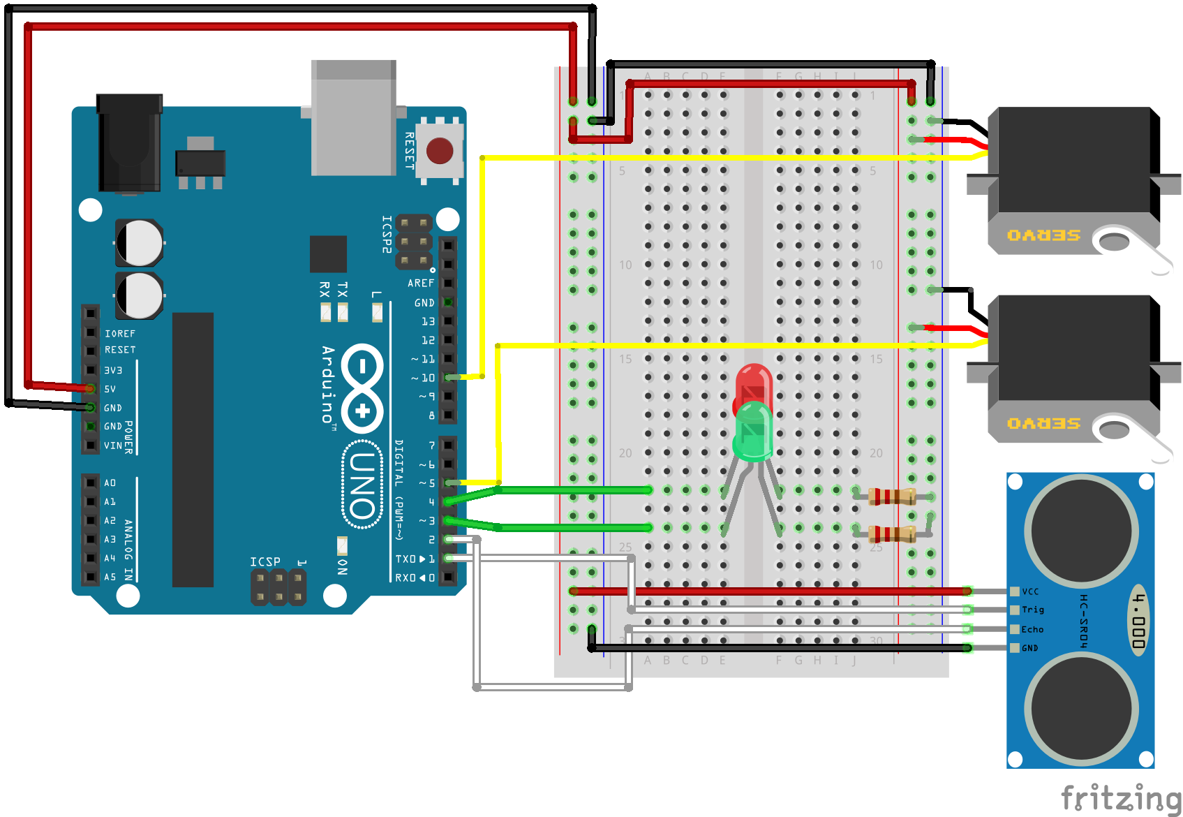
Next, we moved onto attempting to define a more accurate illustration of the data set in regards to the context of the problem, renewable energy usage. We decided the best way to do this was to put everything in terms of the estimated amount of pollution each state was producing per year. We determined this value for each state per year by calculating the summation of each states energy consumption value multiplied by the transfer rate between that specific energy type and CO2 emissions. Essentially, we arranged Jet Fuel, Natural Gas, Coal, Petroleum, Motor Gasoline, and LPG consumptions per year in a single-column matrix and found its dot product with a constant single-column matrix that consisted of the conversion coefficients for that specific energy type and CO2 emissions, labeled C in the graphic below. We determined the conversion coefficients by pulling data from the EIA (here).

Screen Shot 2018-02-19 at 2.08.00 PM.png

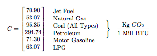
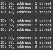
Screen Shot 2018-02-19 at 2.09.34 PM.png Excerpt from our final paper detailing the values of the C conversion constant and giving Arizona’s numbers for 2009.

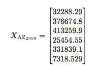
Using the information above (Note: the structure of X_AZ follows that of C (in order of energy type from top to bottom, given in billion BTU. A conversion factor of 1000 Mill BTU / 1 Bill BTU was added) we are able to calculate an estimation of the CO2 emissions in Arizona in 2009 (X_AZ_2009 * C = 93307874.83 metric tons of CO2. Given the population of Arizona in 2009, we can then determine an estimation of CO2 emissions per capita of Arizona in 2009 (abt. 14 metric tons of C02 per capita). We then generalized this process in order to create a graph of CO2 emissions in each state per year.

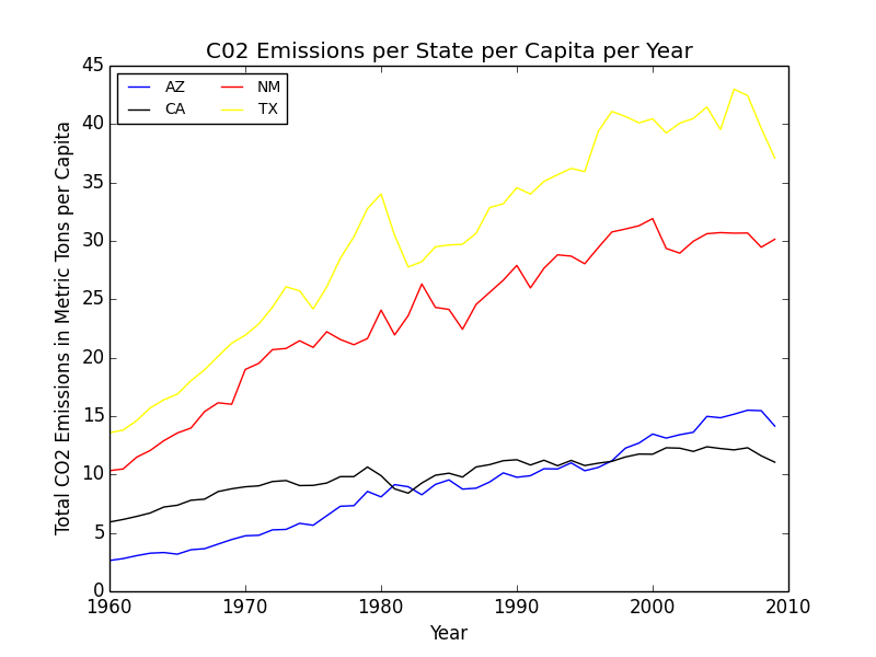
Graph detailing CO2 emissions per capita per year in each of the states. We used this information to generally rank each state in terms of pollution production, in order to circle back and create a discussion surrounding using cleaner energy sources.

Next came predicting energy consumption/production in 2025 in the context of cleaner energy usage. For this, as we began to run out of time (we only had four days for this competition) we resorted to using a basic linear regression to predict the values for 2025 and 2050. The main notable conclusion from this experiment was seeing how high energy consumption values were predicted to become, especially in regards to the very rapidly increasing CO2 emissions per capita for each state. As an example, total energy consumption in Arizona, using the linear regression model, was projected to increase by over 800,000 BTU. This, paired with the estimated increase in CO2 emissions per capita of abt. 5 metric tons per capita shows just how quickly pollution is projected to get out of control. Of the four states, Texas had the worst CO2 emission rates per capita estimated by 2050, seeing an increase of 37 metric tons per capita from 2009 (a projected value of abt 76 metric tons per capita). Again, we used these values to stress the importance of switching to more renewable energy sources in the coming years, before damage becomes irreversible.

Using all of the above data, we discussed in our conclusion the importance of moving away from commonly-used, bad for the environment energy sources. With the exponential increase in population in all of these states and really throughout the world, energy consumption and production has understandably seen a drastic increase in recent years. However, with the threat of global warming, each state needs to do whatever it can in order to slow or even reverse the effects brought on by these increased consumption and production rates.

I’m incredibly thankful to have competed in the GDMS competition prior to this competition, because without prior experience, we definitely would have had no idea where to start and probably would not have finished on time (of which we only barely did given the work detailed above, after making a numerous amount of assumptions ultimately weakening our argument). All in all, this competition was equally taxing on our mental health as it was fun to compete in. We look forward to participating in future data analysis competitions in the future. Unfortunately, we don’t hear back about the results until some time in April. If you want to see our final paper (written in LaTeX) in detail, you can find it here.

2018 Winter AI Project – Connect 5 Minimax

February 5, 2018 / mccloskeybr / 1 Comment

After finishing my previous project, I still found myself with plenty of time in-between classes (thankfully I’m only taking 4 courses this semester as opposed to my usual 6, so hopefully this trend continues throughout the semester). Also, as I recently took up a UTA position for CS2505 at VT (Intro to Comp Org), I found myself with plenty of down time on-shift as the early assignments are easy and most students don’t need help as of yet. Thankfully, some friends come and spend time with me to make the time go by faster. One of these friends typically brings a Go board along with her and loves to play connect 5 with us (think tic-tac-toe, but on a Go board, and you have to connect 5 instead of 3). After countless games, I thought back to my minimax algorithm for tic-tac-toe (here), and wondered if it applied smoothly to connect 5. And so, I decided to start working on this project.

First was to create the game. I was drawn to Java because I’m most comfortable working with object-heavy projects in Java (as opposed to something like Python). Coding the basic game was simple. The board itself is basically an 18×18 tic-tac-toe board. As such, I just used a 2D integer array size 18×18 and used constants for black, white, and empty spaces. I used swing for rendering, and KeyListeners for user input. Arrow keys navigate and enter places a piece. Upon placing a piece, control is handed over to the AI to decide the move they are going to take.

Screen Shot 2018-02-05 at 2.24.53 PM.png
Empty gameboard. The cursor is indicated with the red square (moves with arrow key input). As you’ll see later, the blue cursor (not shown here) indicates the previous move.

Next came calculating the heuristics for scoring any given board. I used this post by Ofek Gila as a foundation and built on that. Essentially, the board is traversed in every direction (horizontal, vertical, topleft->bottomright diagonal, topright->bottomleft diagonal) and consecutive pieces are counted and scored, with the sum total being the overall score of the current board state. The scores for consecutive pieces are based on the perceived value of that shape (i.e. a 5 in a row is worth much more than a single piece). I wanted this version to play very defensively (an annoying strategy for veterans of the game), so there are noticeable score differences based on what the color of the consecutive pieces is. Afterward, I began writing the minimax algorithm. The basic jist of minimax is to look a set number of moves into the future, score the current board state, and play off of the assumption that your opponent is going to make the best move for them at their given board state (hence the name minimax — you’re trying to maximize your gains and the opponent is trying to minimize them). I settled on looking 2 moves into the future, as it fit the balance of running quickly and decent decision making. If you want to learn more about minimax, feel free to look at the code for this project (link at the bottom).

Screen Shot 2018-02-05 at 2.23.14 PM.png
Using minimax, the AI (white) was able to defeat the user (black) here, while also stopping a win for black (if the white piece at the upper-right was not placed, black would have won)

Using this method, I ran into a couple of speed bumps. The major issue was performance. Especially at the beginning of the game, even after the user’s move, there are still 323 possible moves (18^2=324, -1 for the placed piece). That in addition to looking n moves into the future, meant that there are about 323^n checks that the algorithm needs to make (the number is actually slightly less than 323^n, as it doesn’t factor in placing new pieces and repeating the process, but it is essentially that value for small values of n, so we will ignore it for this basic analysis). To solve this, I cropped the board down to only ‘relevant’ spaces (I defined relevant here as any space around all of the current pieces in play with a buffer of 2 spaces on every side). Using this method, I was able to reduce the number of checks for 2 moves from 323^2=104,329 to 25^2=625 (placing one piece and creating a buffer of size 2 on every side creates a 5×5 grid, resulting in the 25 seen there (5^2 = 25)). Other than that, there is a bug in which the AI would let the player win if it won later down the decision-tree (in other words, it detected a win but didn’t take into account the opponent winning sooner). I expect this to be an error with scoring, but as I want to continue working on other projects, I will leave this bug in for now.

Screen Shot 2018-02-05 at 2.21.13 PM.png
You can see that the AI (white) detected a win, so it ignored black’s 3 in a row, ensuring a win for black.

Testing this out on some of my friends, I found that it played fairly decently. However, due to some minor bugs in the score evaluation (detailed at the end of the previous paragraph), veterans could consistently beat the bot (albeit after hard, long-fought games). This project was a fun one that I could share with friends, so I definitely enjoyed working on it and seeing it get better along the way. I encourage you to download the project and try playing against it yourself. You can find the github for this project here.

2018 Winter Web Project – Pyreddit

January 23, 2018 / mccloskeybr / 0 Comments

During the start of my spring semester, I found myself with a lot of free time while waiting for classes to pick up in difficulty. I thought of side projects to do to fill up this time, and decided to focus on something web-based, as the last time I did anything web related was in highschool. Eventually, I ended up finding projects like rtv, of which inspired me to create something of a reddit browser from terminal. Upon doing a bit of research, I found that there exists a nice, easy to use library that handles connecting to reddit in python called praw. I mainly focused on browsing, not submitting jobs (like upvoting or writing a post), simply because I focused on my own reddit-using habits. I mainly read posts, and rarely (if ever) make them, so I decided to cut that feature from my program. Perhaps if I come back to this in the future, I will implement those features.

Thanks to praw, connecting to reddit was very easy. Given some credentials (along with authorization codes for a script to connect to reddit), I was able to connect in essentially just one line. Praw allows easy movement within reddit as well, whether it be connecting to different subreddits or posts within a subreddit, its all very easy and straightforward. If you’re considering making any script or application that will connect to reddit, I strongly recommend praw. View connection_manager.py (github linked below) to see for yourself how easy everything really was.

Screen Shot 2018-01-23 at 3.00.49 PM.png
All of the setup for pyreddit occurs within less than a second, and is easy to implement from a developer’s point of view.

Other than establishing a connection, all that was left was figuring out how I wanted to do the user interface. I used the colorama library to color text, and used reddit’s basic layout as inspiration for the various aspects that needed a ui. First off was subreddits. Praw loads in an iterator for a large number of posts from a given subreddit and tab (hot, top, new, etc.) so all I needed to do was separate those into pages.

Screen Shot 2018-01-23 at 3.03.40 PM.png
Cutout of a page in pyreddit. I tried to make each bit of information color-coded to ease user understanding. If the user wants to open one of these posts, they simply have to type ‘open i‘, where i is the index of the post (shown in red in the screen).

Next was creating an interface for posts. I created a simple method for breaking text bodies into chunks that were easy to read (split the post body at the space after 100 characters from the previous split) and created comment trees similar to that of python using depth-first search. All of which resulted in a simple, clean style that doesn’t look too bad. I used the webbrowser library (standard in python) to open the current post’s url if so desired as well.

Screen Shot 2018-01-23 at 3.10.37 PM.png
Example of a post shown within pyreddit. If the post itself contains a body, it is printed in the same fashion (split every 100 characters at a space, etc.)

This was a quick and easy project that helped me further my understanding in python scripting and establishing web connections (esp. to reddit). If you want to download this program or look at the code, you can find the github for this project here.

2015 Winter Cryptography Project – P / NP, The Clique Problem

January 13, 2016 / mccloskeybr / 0 Comments

I recently read a book titled The Golden Ticket by Lance Fortnow in which the P / NP Problem and its importance to the theory of Computer Science are heavily discussed. Explained briefly, the P / NP Problem asks if every single problem can be solved quickly and efficiently. In relations to cryptography, P / NP is crucial because it allows for the creation of hard math problems to, for example, be able to hide private information on a public network. One of the most famous P / NP Problems, the Clique problem, was discussed and is, in my opinion, one of the more intriguing problems in the book.

Take, for example, a society called Frenemy, in which every citizen either has a 50% chance to be friends or a a 50% chance to be an enemy with a person they just met. In Fortnow’s book, he details how it would be virtually impossible to find all cliques of varying sizes (difficulty/time to find all cliques increases as size of desired clique increase) inside of this society (A clique is a group of people in which everyone is friends with all other members). At first, I didn’t think it would be that difficult to find the largest clique, but after making a simulation for myself, I was proven otherwise.

I stayed true to the Frenemy rules in my simulation – every time someone meets someone else, they have a 50% chance to either be their friend or their enemy. I experimented with varying population sizes as well as varying amounts of citizens in which each person can meet. I made two methods in order to experiment, one in which everyone meets everyone else in the society, and one in which everyone meets everyone on their own street (9 total streets in which 1/9 of the total population lives on each given street). To make the data easier to set up and understand, each citizen is given an identification number as well as an ‘address’, the number of street they live on. I aimed to find every single clique of size 3 in the society, and to see for myself how difficult it became to find them as population size increased.

Screen Shot 2016-01-13 at 1.49.10 PM

A couple of cliques present in a population size of 100 in which citizens met everyone on their own street.

I found that the total time to generate the population and find cliques of size 3 took much much longer the higher the population size was, which makes sense in hindsight. Adding a single citizen to a population size of 20 where everyone meets everybody doesn’t have nearly the impact as adding a citizen to a population size of 10,000, as the number of updates a computer has to make to each citizen’s list of friends and enemies for a population of 10,000 is much larger. When I was reading Fortnow’s book, I didn’t put much thought into the rate at which the updates change as population size grows. I naively thought growth was generally linear, allowing total computations to find all cliques of size 3 to be relatively small compared to the actual value. Only after I made my own simulation did I truly understand the difficulty surrounding finding a solution to the Clique problem. If you find find yourself with some free time, I would recommend making a simple simulation like this for yourself so you can see the results firsthand.

I’d like to thank Lance Fortnow for pushing me to explore this problem through his book, as all P / NP problems (not just the Clique problem) are profoundly interesting in their own rights. And, if you’re planning to look more into the P / NP problem, Lance Fortnow’s The Golden Ticket is a must read. The discussion as well as the existence of the P / NP Problem has really expanded my understanding of Computer Science and the importance of not only the physical act of coding, but the theory behind CS as well.

2015 Winter AI/Arduino Project – Brainy Crawler

January 12, 2016 / mccloskeybr / 0 Comments

Having taken a general engineering course my senior year of High school at the same time I was researching Neural Networks (read more about Neural Networks here), I decided it was time to make a physical agent – a tangible robot controlled by a Neural Network. My background in robotics helped in this venture as well, as I knew before hand how servos and ultrasonic sensors worked.

Before getting to the hard part of writing the code to control the robot, I had to make the agent itself first. I knew I wanted to make a robot that learned how to move, but I didn’t have 2 motors. Instead, I decided to use servos, as it not only allows movement, but the motion itself is complex and warrants a fair amount of learning in order to master it. For parts, I used an Arduino Uno with 2 Parallax standard servos and 1 HC-SR04 Ultrasonic sensor. A friend of mine, Clay Busbey, helped out by 3D printing parts for me. I had 3 parts printed, the main chassis and 2 essentially straight bars used as 1 arm with a joint. I put the Arduino Uno and a half+ breadboard onto the chassis and hooked everything up from there.

crawler_png

Fritzing diagram of how I hooked up all of the components. It doesn’t show the bars used for arms, but you’ll see how that works in the next gif. The red and green LEDs indicate whether the Arduino is switching between Networks, red meaning it’s switching, and green meaning movements are controlled by a Neural Network.

In terms of the Neural Network, I used 3 input nodes, 1 hidden layer of 10 nodes, and 2 output nodes. The input values are the current position of each servo, along with the current distance away from the object detected in the ultrasonic sensor. The output values decide whether the servo should increase or decrease its current angle (> or < 0.5). I used a sigmoid function (1 / (1 + e^(-x))) as my activation function. Each Neural Network controls one motion, with a genetic algorithm that replaces the least successful Network (2 best networks make a crossover/mutation child that replaces worst network). Fitness is distributed based on how far the robot moved while under control of each Neural Network.

brainy crawler

Timelapse of the agent moving across the floor (sped up 3x). You can see that although it has a good start, it hiccups due to either a bad breed or mutation.

I enjoyed working on this project. It’s really one thing to watch a program learn in the real world as opposed to in the virtual world.

If you want to get the Arduino script and/or the .stl files for 3D printing the parts, you can get them here (.zip, 15 kb): https://drive.google.com/file/d/0Bz_0wgRmDpKqdGdGUS1YMk9oN1E/view?usp=sharing

2015 Winter AI Project – Evolution Simulator

January 5, 2016 / mccloskeybr / 0 Comments

The 2015 school year was when I began dabbling around AI. The idea always amazed me. Everything from movie depictions of them to the real practical uses they have in modern day life was interesting, and I wanted to know more about it.

Wanting to explore Neural Networks deeper (read more about Neural Networks here), I decided to make an evolution simulator. The aim of the project was to create a population of creatures that, starting with knowing nothing about their environment, evolved to chase after food and run away from predators. The creatures can also evolve different values of attack and defense, of which determines if that creature can eat other creatures. A set of 12 creatures is allowed to survive for as long as it can (must eat food to replenish a diminishing energy value, if it gets to 0 the creature dies), and at the end of the generation, the bottom half is eliminated, the top half reproduces sexually once (2 children) with each other (first mates with second, third mates with fourth, and so on), and asexually once as well. Reproduction is accomplished with crossover/mutation, that takes into account the weights for each creatures Neural Network and the attack value for each creature. Fitness is distributed based on how many times the creature eats.

The Neural Network itself was fun to make. I decided I wanted to make an adaptable system, that is, one in which I can change whenever I want it to. This includes the size of each individual layer and the total amount of hidden layers. For this project, I got the most success using one and two hidden layers with different amount of nodes for each (18 nodes for 1 layer, 5 nodes for 2 layers).

The input for each creature is as follows: 2 ‘eyes’ that take up 4 input nodes, as well as one node expressing the current angle the creature is facing. Each eye detects the angle from the creature to the closest entity (or second closest, for the second eye) and the r, g, and b values of that entity, expressed as a fraction over 255 (the range a color value can have is [0, 255]), allowing the creature to evolve decision making based on whether the entity it sees is edible or not. The output nodes control whether it turns left or right, and its velocity forwards or backwards (move more slowly while going backwards). I used a sigmoid function (1 / (1 + e^(-x))) as my activation function.

Screen Shot 2016-01-05 at 10.12.19 AM

Neural Network that has 9 input nodes, 1 hidden layer with 18 nodes, and 2 output nodes. The color for each weight is explained below.

Before I go over examples of the simulation, I’ll explain what each of the graphics in the frame represent. The creatures are represented by shades of purple (creatures that have a high defense are more blue while creatures that have a high attack are more red), with the current best creature (highest fitness) is outlined in yellow. The line extending from the center from each creature to its outline is the direction in which the creature is currently facing. Food is represented by the green squares. Moving onto the panels outside the main frame, the one in the top right shows the current generation, the amount of creatures alive (from a set max population size of 12), the best fitness value from the overall simulation, the best fitness value from the previous generation, and the best fitness for the current generation (represented with O, LR, and C respectively). The graphic below that panel displays the Neural Network of the creature that garnered the best fitness, where connections that are mostly red are between (0, 1), and connections that are mostly blue are between (-1, 0). Finally, the graph displayed on the bottom of the frame illustrates the best fitness for each round and shows overall growth of the population.

beginning

At the beginning, you can observe how most creatures are spinning out of control and lack in objective.

structured

After some time, you can see that although the creatures have not evolved the ability to go directly towards food, they have formed some structure in the way they collect it. You can also see that this population has evolved to contain creatures that have a high defense, as creatures that had a high attack in previous generations did not perform as well.

end usual

The usual ending. Creatures have evolved to not only go towards food, but to distinguish food from other creatures. That means that although an entity might be closer and thus more efficient to go towards, the creatures recognizes that entity as another creature and decides to go towards an entity that is further away because it recognizes that as food.

ending weird

Although creatures tend to evolve the ability to go straight for food, there are other strategies that have the possibility to emerge. For instance, in the simulation above, the creatures have come up with the strategy to propel themselves vertically, turn horizontally, and propel themselves the left or right whenever they detect food.

This project was incredibly fun to make. Although I had some frustration at the start while learning how to make Neural Networks of varying size, it was fun finding solutions to my problems. I will probably keep working on this project for weeks or months to come, and I will definitely be utilizing my adaptive Neural Network on future projects.

If you want the source code, you can get it here (Java, 35 kb): https://drive.google.com/file/d/0Bz_0wgRmDpKqaXV0TVp0aXhIcTA/view?usp=sharing

2015 Winter AI Project – Wall Avoider

December 23, 2015 / mccloskeybr / 0 Comments

During the holiday break, I decided to dedicate my programming efforts towards learning Neural Networks. I knew a little bit about them before hand, like the architecture and the theory of how they worked, but had no idea how to implement them into my own projects. The wall avoider project was dedicated towards making a very, very simple Neural Network that progressively got better at avoiding walls using a genetic algorithm.

But first, I will briefly explain what Neural Networks are. In short, they are systems modeled after the human brain – that is, they use a set of ‘neurons and synapses’ that manipulate a given set of input data so that a desired output is reached. The issue is, however, that we do not know the correct weights and values necessary so that the network will give us our desired output. There are several ways of determining error/finding the best set of values so that a desired output is reached. For this project, I’ll be using a genetic algorithm to essentially determine the best network, and ‘breed’ it with other good networks, resulting in an equally if not better Neural Network. This occurs by choosing 2 Neural Networks that result in a long run (doesn’t hit the wall) and randomly choosing weights from both networks to result in a new Neural Network.

neural-network

Anatomy of a Neural Network.

My project’s Neural Network has 3 input nodes and 1 output node. The value of the input nodes is either a 1 or a 0, depending on whether or not its respective ‘eye’ (line extending from the center of the runner) hits a wall or not. These values are each multiplied by their respective weights (random at first, then altered through the genetic algorithm) and summed together, then put through an activation function. In my example I used a variation of a sigmoid function (1 / (1 + e^(-x)) as an activation function. Sigmoid functions are nice because their ranges are typically (0,1), resulting in either an ‘on’ or an ‘off’ setting. If the a(x) > 0.5, it turned right. If a(x) < 0.5, it turned left. If a(x) = 0.5, it didn’t turn at all.

Screen Shot 2015-12-23 at 12.47.08 PM

Graphic of my Neural Network. i = input (eyes), W = weights, a = activation

After constructing this system, I began running tests. As the objective wasn’t a hard one to learn, the networks involved mastered the challenge quickly. In the gifs, you can see on the left the trial number and the fitness value (how well the network is doing) for each member of the population. p# = parent, c = child, and ^ indicates current best network.

trial 1

Trial 1, struggling.

trial 7

Trial 7, a pretty decent network is bred, but still room for improvement.

trial 25

Trial 25, all networks are doing very well.

This was a great intro to Neural Networks. I definitely want to take this idea further and create deeper, more complex networks for harder tasks.

If you want the source code, you can get it here (Java, 26kb): https://drive.google.com/file/d/0Bz_0wgRmDpKqSVRvbXpzcm1VRVE/view?usp=sharing

2015 Winter AI Project – Maze Runner

December 18, 2015 / mccloskeybr / 0 Comments

After my Chess project, I wanted to become a little more serious in my research surrounding artificial intelligence. I looked up everything from examples of how it was used in day to day life to videos of lectures by college professors. I learned a lot about the concept of reinforcement learning through these lectures and even watching college Thesis projects, making me want to program something to test out the idea.

First, however, a very brief overview of my current understanding of reinforcement learning. Reinforcement learning is a system in which the AI learns about the environment it’s put in through a system of actions and states. The ai is rewarded or punished through the various states (depending on whether you want to maximize utility or minimize cost, either way is fine, but for my example I will be using a reward system) for good actions versus bad actions, but the AI doesn’t know which actions are good or bad until it experiences them. Thus, after a long time, the AI should begin to gravitate towards actions that garner it the largest sum reward.

Alright, now to my project. I decided to go with something simple and intuitive to explore the concept of reinforcement learning through creating an artificial intelligence that would find the quickest path to an exit in a predefined maze. As mentioned before, the AI started with knowing absolutely nothing about the maze it was placed in, and must learn everything from scratch.

Screen Shot 2015-12-18 at 2.09.06 PM

Original board displaying reward values for each tile (currently 0 because the AI doesn’t know which tiles are good and bad yet). The blue tile is the current position of the runner (controlled by the AI) and the green tile is the exit.

The reward system for the AI essentially takes in all of the rewards of the tiles it visited and sums it together, divides that number by the amount of tiles visited, and uses that value to update the reward value for all of the tiles it visited. The tiles takes that value and averages it into all of its previous rewards given from previous trials. The AI gets a heavy reward boost for completing the maze faster than before, and a heavy punishment if it was slower (increase/decrease overall reward by a factor of 2). Thus, over time, the AI slowly becomes better and better at solving the maze.

The 10th trial. You can see the general path the AI takes (tiles with the highest reward) is rather sporadic.

The 50th trial. The AI has begun to iron out all the kinks in the path, but it isn’t yet the most efficient.

100

The 100th trial. You can see the AI has almost found the most efficient path.

I heavily enjoyed this project, as watching something learn, especially a program, is really interesting. I’m really excited to see where I can take this in the future.

If you want to play around with this, you can get the source code here (Java, 24kb): https://drive.google.com/file/d/0Bz_0wgRmDpKqNUVpTFFQdUNaaUk/view?usp=sharing

Theme by Anders Norén — Up ↑

Brendan McCloskey

software developer

Recent Posts

Recent Comments

Archives

Categories

Meta